In this post, we explore the Iris dataset, a well-known dataset containing information about three Iris species. We start by importing necessary Python modules for data analysis. The dataset includes four numeric attributes for each species: sepal length, sepal width, petal length, and petal width. It contains 150 samples in total and is commonly used for classification tasks.
We check for missing values in the dataset and find that it’s clean, with no null entries. We then calculate summary statistics for the attributes, providing insights into their distribution.
To visualize the data, we create boxplots to compare attribute distributions across the three Iris species. ANOVA tests confirm significant differences in means among the species for all attributes.
A pairplot is generated to visualize relationships between features, helping uncover patterns and correlations. A correlation matrix heatmap illustrates interdependencies between attributes.
Lastly, we use PCA to reduce dimensionality and create a 3D plot, showcasing how well the Iris species are separated in this reduced space. These steps offer a comprehensive exploration of the Iris dataset, aiding in data analysis and visualization tasks.
Contents
- Import modules
- The iris dataset
- Data types
- Null values
- Common statistical values
- Boxplots
- ANOVA (Analysis of Variance)
- Pairplot
- Correlationmatrix
- 3D Plot and PCA reduction
- References
- License
Import modules
import numpy as np
import pandas as pd
import seaborn as sns
from scipy import stats
import matplotlib.pyplot as plt
from mpl_toolkits.mplot3d import Axes3D
from matplotlib.animation import FuncAnimation, PillowWriter
from sklearn.datasets import load_iris
from sklearn.decomposition import PCA
The iris dataset
The Iris dataset, by Sir R.A. Fisher, includes 150 samples of three Iris species, each with four attributes. It’s key for teaching classification algorithms, highlighting linear and non-linear separability. With its balanced and comprehensive data, it’s an excellent introductory dataset for statistical classification.
iris = load_iris()
print(iris.DESCR)
Iris plants dataset
--------------------

**Data Set Characteristics:**

:Number of Instances: 150 (50 in each of three classes)
:Number of Attributes: 4 numeric, predictive attributes and the class
:Attribute Information:
    - sepal length in cm
    - sepal width in cm
    - petal length in cm
    - petal width in cm
    - class:
            - Iris-Setosa
            - Iris-Versicolour
            - Iris-Virginica

:Summary Statistics:

============== ==== ==== ======= ===== ====================
                Min  Max   Mean    SD   Class Correlation
============== ==== ==== ======= ===== ====================
sepal length:   4.3  7.9   5.84   0.83    0.7826
sepal width:    2.0  4.4   3.05   0.43   -0.4194
petal length:   1.0  6.9   3.76   1.76    0.9490  (high!)
petal width:    0.1  2.5   1.20   0.76    0.9565  (high!)
============== ==== ==== ======= ===== ====================

:Missing Attribute Values: None
:Class Distribution: 33.3% for each of 3 classes.
:Creator: R.A. Fisher
:Donor: Michael Marshall (MARSHALL%PLU@io.arc.nasa.gov)
:Date: July, 1988

The famous Iris database, first used by Sir R.A. Fisher. The dataset is taken
from Fisher's paper. Note that it's the same as in R, but not as in the UCI
Machine Learning Repository, which has two wrong data points.

This is perhaps the best known database to be found in the
pattern recognition literature.  Fisher's paper is a classic in the field and
is referenced frequently to this day.  (See Duda & Hart, for example.)  The
data set contains 3 classes of 50 instances each, where each class refers to a
type of iris plant.  One class is linearly separable from the other 2; the
latter are NOT linearly separable from each other.

|details-start|
**References**
|details-split|

- Fisher, R.A. "The use of multiple measurements in taxonomic problems"
  Annual Eugenics, 7, Part II, 179-188 (1936); also in "Contributions to
  Mathematical Statistics" (John Wiley, NY, 1950).
- Duda, R.O., & Hart, P.E. (1973) Pattern Classification and Scene Analysis.
  (Q327.D83) John Wiley & Sons.  ISBN 0-471-22361-1.  See page 218.
- Dasarathy, B.V. (1980) "Nosing Around the Neighborhood: A New System
  Structure and Classification Rule for Recognition in Partially Exposed
  Environments".  IEEE Transactions on Pattern Analysis and Machine
  Intelligence, Vol. PAMI-2, No. 1, 67-71.
- Gates, G.W. (1972) "The Reduced Nearest Neighbor Rule".  IEEE Transactions
  on Information Theory, May 1972, 431-433.
- See also: 1988 MLC Proceedings, 54-64.  Cheeseman et al"s AUTOCLASS II
  conceptual clustering system finds 3 classes in the data.
- Many, many more ...

|details-end|
This Python code snippet enriches the Iris dataset by adding a categorical column for species, converting numerical codes to readable species names. The output shows the first five rows, all labeled “setosa,” one of the three species in the dataset alongside “versicolor” and “virginica.” This approach simplifies data analysis, making the dataset immediately more accessible and interpretable for various tasks, including machine learning and statistical analysis.
pd.set_option('display.max_columns', None)

iris_df['species'] = pd.Categorical.from_codes(iris.target, iris.target_names)

print(iris_df.head())
sepal length (cm)  sepal width (cm)  petal length (cm)  petal width (cm)  species
0             5.1               3.5                1.4               0.2  setosa
1             4.9               3.0                1.4               0.2  setosa
2             4.7               3.2                1.3               0.2  setosa
3             4.6               3.1                1.5               0.2  setosa
4             5.0               3.6                1.4               0.2  setosa
Data types
This code snippet demonstrates how to load the Iris dataset and create a pandas DataFrame from it, naming the columns according to the dataset’s feature names: sepal length, sepal width, petal length, and petal width, all measured in centimeters. The dtypes method reveals that each of these columns is stored as float64 data type, indicating that all the measurements are represented as floating-point numbers. This data type choice is appropriate for continuous numerical data, facilitating various data analysis and machine learning tasks that require numerical input.
iris = load_iris()
iris_df = pd.DataFrame(data=iris.data, columns=iris.feature_names)

print(iris_df.dtypes)
sepal length (cm)    float64
sepal width (cm)     float64
petal length (cm)    float64
petal width (cm)     float64
dtype: object
Null values
By examining the Iris dataset for missing values, the output reassuringly confirms that every column—sepal length, sepal width, petal length, petal width, and species—has zero missing entries. This level of data integrity simplifies preprocessing steps, allowing for straightforward analysis and application in machine learning models, as it negates the need for initial data cleaning to address null values.
print(iris_df.isnull().sum())
sepal length (cm)    0
sepal width (cm)     0
petal length (cm)    0
petal width (cm)     0
species              0
dtype: int64
Common statistical values
Exploring the Iris dataset through its statistical summary provides a clear picture of the floral dimensions it encompasses. The average sepal length is about 5.84 cm, while the average petal length is notably shorter at 3.76 cm, illustrating the variation in flower morphology. With sepal widths averaging at 3.06 cm and petal widths at 1.20 cm, the dataset captures a detailed snapshot of Iris plant characteristics. The range of values, from the shortest petal at 1.0 cm to the longest sepal at 7.9 cm, showcases the diverse sizes within the Iris species. This summary not only offers a quick glance at the dataset’s features but also hints at the intricate patterns that could be explored in predictive modeling and data exploration efforts.
iris = load_iris()
iris_df = pd.DataFrame(iris.data, columns=iris.feature_names)
iris_df['species'] = pd.Categorical.from_codes(iris.target, iris.target_names)

print(iris_df.describe())
       sepal length (cm)  sepal width (cm)  petal length (cm)  petal width (cm)
count         150.000000        150.000000         150.000000        150.000000
mean            5.843333          3.057333           3.758000          1.199333
std             0.828066          0.435866           1.765298          0.762238
min             4.300000          2.000000           1.000000          0.100000
25%             5.100000          2.800000           1.600000          0.300000
50%             5.800000          3.000000           4.350000          1.300000
75%             6.400000          3.300000           5.100000          1.800000
max             7.900000          4.400000           6.900000          2.500000
Boxplots
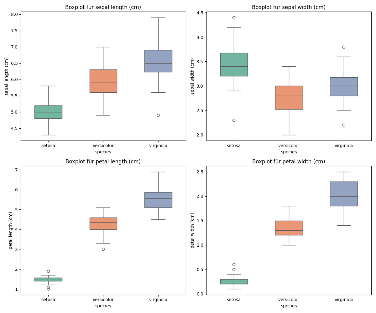
This Python code block creates a series of boxplots for the Iris dataset, visually comparing the distributions of sepal length, sepal width, petal length, and petal width across the three Iris species: Setosa, Versicolor, and Virginica. Using the seaborn library for plotting, each feature’s boxplot is categorized by species, with a different color for each species from the “Set2” palette for clarity. The dodge=False parameter ensures the boxplots are aligned directly above their corresponding species categories on the x-axis, and the width=0.5 parameter adjusts the boxplots’ width for better visualization.
By iterating over the feature names and creating a subplot for each, the code neatly organizes the visual comparison into a 2x2 grid, making it easy to observe differences between species for each measured attribute. The titles are dynamically set to reflect the feature being plotted, enhancing readability.
Finally, the use of plt.tight_layout() adjusts the spacing between plots to prevent overlap, ensuring that each plot and its title are clearly visible. The resulting figure is then saved as “boxplots_iris.png”, providing a useful visual reference that can aid in understanding species differences based on morphological measurements within the Iris dataset.
plt.figure(figsize=(12, 10))
for i, feature in enumerate(iris.feature_names):
    plt.subplot(2, 2, i+1)
    sns.boxplot(x='species', y=feature, hue='species', data=iris_df, palette="Set2", dodge=False, width=0.5)
    plt.title(f'Boxplot für {feature}')

plt.tight_layout()
plt.savefig("boxplots_iris.png")
ANOVA (Analysis of Variance)
Now we perform an ANOVA (Analysis of Variance) test on the Iris dataset to compare the means of sepal length, sepal width, petal length, and petal width across the three Iris species: setosa, versicolor, and virginica. ANOVA is used to determine if there are any statistically significant differences between the means of three or more independent groups.
The results show a high F-value and a very small p-value for each feature, indicating strong statistical evidence that at least one species mean is different from the others for each of the four features measured. Specifically:
For sepal length, the F-value is about 119.26 with a p-value near zero (1.67e-31), suggesting significant differences in sepal length among the three species. Sepal width also shows significant differences, with an F-value of 49.16 and a p-value of 4.49e-17. Petal length and petal width present even more pronounced differences, with F-values of 1180.16 and 960.01, respectively, and p-values essentially zero (2.86e-91 for petal length and 4.17e-85 for petal width). These findings underscore the morphological diversity among Iris setosa, versicolor, and virginica, reinforcing the suitability of these features for species classification tasks. The very low p-values across all features confirm that the differences in means are not due to random chance, highlighting the distinctiveness of each species in terms of their floral measurements.
for feature in iris.feature_names:
    setosa = iris_df[iris_df['species'] == 'setosa'][feature]
    versicolor = iris_df[iris_df['species'] == 'versicolor'][feature]
    virginica = iris_df[iris_df['species'] == 'virginica'][feature]

    f_value, p_value = stats.f_oneway(setosa, versicolor, virginica)
    print(f"ANOVA für {feature}: F-Wert = {f_value}, p-Wert = {p_value}")
ANOVA for sepal length (cm):       F-Wert = 119.26450218450468,       p-Wert = 1.6696691907693826e-31
ANOVA for sepal width (cm):        F-Wert = 49.160040089612075,       p-Wert = 4.492017133309115e-17
ANOVA for petal length (cm):       F-Wert = 1180.161182252981,        p-Wert = 2.8567766109615584e-91
ANOVA for petal width (cm):        F-Wert = 960.007146801809,         p-Wert = 4.169445839443116e-85
Pairplot
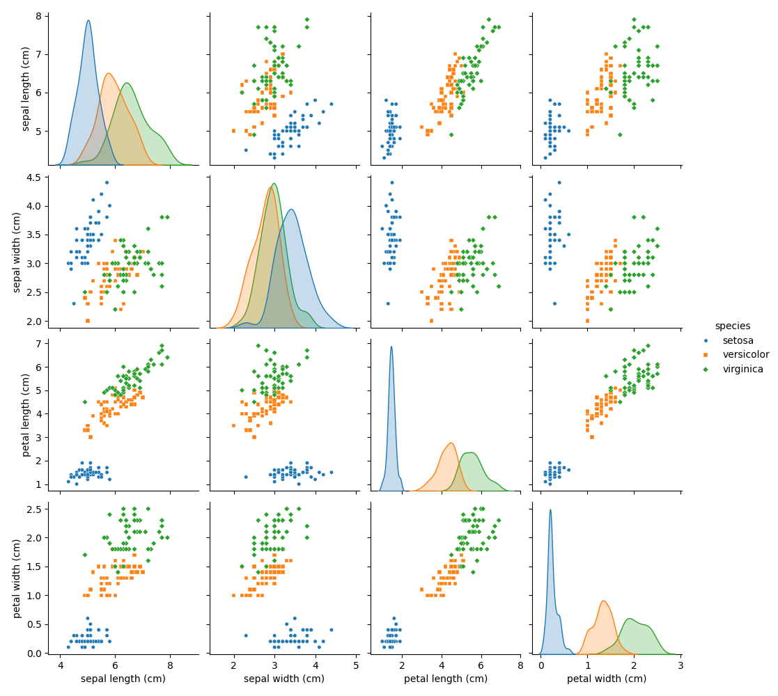
Creating a pairplot of the Iris dataset unfolds a visual narrative that deeply explores the interplay between the dataset’s features. By converting the species into categorical labels and mapping these alongside the Iris measurements, we illuminate the nuanced distinctions and patterns among the species. This visualization technique, adeptly applied through seaborn, leverages hues and marker shapes to differentiate between Iris-Setosa, Iris-Versicolor, and Iris-Virginica, offering a canvas where the intricate dance of data points tells the story of biological diversity.
This crafted visual, saved as “pairplot.png”, does more than merely depict data; it invites us into a dialogue with the dataset, revealing clusters and correlations that might not be immediately apparent. It showcases how the dimensions of sepal and petal measurements intersect across species, serving as a foundational tool for both exploratory data analysis and the preliminary assessment of features for classification tasks. Through this lens, the Iris dataset is not just a collection of numbers but a testament to the power of statistical visualization in uncovering the hidden patterns that reside within.
iris = load_iris()
iris_df = pd.DataFrame(iris.data, columns=iris.feature_names)
iris_df['species'] = pd.Categorical.from_codes(iris.target, iris.target_names)

sns.pairplot(iris_df, hue='species', markers=["o", "s", "D"],
             plot_kws={'s': 15})

plt.savefig("pairplot.png")
plt.show()
Correlationmatrix
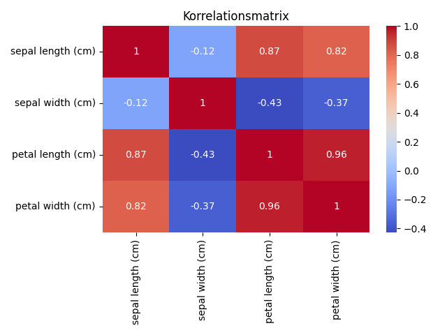
Now we carry out a correlation analysis on the numerical characteristics of the data set. The resulting correlation matrix is like a map of the relationships between the characteristics. Positive values on this map indicate positive correlations, while negative values indicate negative relationships. These numbers are the key to uncovering the hidden patterns in our data. The correlation matrix shows us how strongly the characteristics are interdependent.
numeric_data = iris_df.select_dtypes(include=[np.number])
print("\nCorrelationmatrix (all values):")
pd.set_option('display.max_columns', None)
pd.set_option('display.max_rows', None)
print(numeric_data.corr())
Correlationmatrix (all values):
+-------------------+-------------------+-------------------+-------------------+
| sepal length (cm) | sepal width (cm)  | petal length (cm) | petal width (cm)  |
|-------------------+-------------------+-------------------+-------------------|
| 1.000000          | -0.117570         | 0.871754          | 0.817941          |
| -0.117570         | 1.000000          | -0.428440         | -0.366126         |
| 0.871754          | -0.428440         | 1.000000          | 0.962865          |
| 0.817941          | -0.366126         | 0.962865          | 1.000000          |
+-------------------+-------------------+-------------------+-------------------+
Now let’s look at the generated heatmap, which displays these correlation values in a visually appealing form. In the world of data visualisation, the heat map is like a vivid painting that shows us the patterns and connections between the features.
The heatmap clearly shows that sepal length and petal length have a strong positive correlation. This means that longer sepals tend to have longer petals. There is also a strong positive correlation between petal length and petal width. These findings are valuable to better understand the data structure and can help in the selection of features for analyses or classification tasks.
sns.heatmap(numeric_data.corr(), annot=True, cmap='coolwarm')
plt.title('Korrelationsmatrix')
plt.tight_layout()
plt.savefig("correlation_matrix_iris.png")
3D Plot and PCA reduction
In this code, we try to visualise the relationships between the characteristics of the iris flowers in a three-dimensional space.
Here is a step-by-step explanation:
First, the data is loaded and split into a feature matrix (X) and the corresponding target variables (y). This makes it possible to analyse the characteristics of the iris flowers and understand their relationships.
Principal component analysis (PCA) is applied to reduce the dimensionality of the data to three principal components. This is important to be able to visualise the data in a three-dimensional space while retaining the essential information.
The mean values of the PCA components for each species (Setosa, Versicolor, Virginica) are calculated. These mean values represent the centres of gravity of the data points of each species in three-dimensional space.
The actual 3D data visualisation then takes place. Each iris species is displayed in its own colour (blue for Setosa, green for Versicolor, red for Virginica). The data points of each species are placed in 3D space.
To clarify the separation between the species, two layers are added, one in purple and one in orange. These planes are based on the calculated mean values of the PCA components and help to better understand the spatial distribution of the species.
The interpretation of the data in the plot shows how well the different iris species are separated from each other in three-dimensional space using the PCA components. The clear separation of the species in this space illustrates that PCA is an effective method for reducing the dimensions and provides important information about the data structure.
# Load the Iris dataset using the load_iris function
iris = load_iris()
X = iris.data  # Extract features from the dataset
y = iris.target  # Extract target labels from the dataset

# Apply PCA (Principal Component Analysis) to reduce the data to 3 dimensions
pca = PCA(n_components=3)
X_reduced = pca.fit_transform(X)

# Calculate the means of PCA components for each species in the dataset
means = [np.mean(X_reduced[y == species, :], axis=0) for species in range(3)]

# Create a 3D plot to visualize the reduced data
fig = plt.figure(figsize=(10, 7))
ax = fig.add_subplot(111, projection='3d')

# Plot each species separately with distinct colors
colors = ['blue', 'green', 'red']
labels = ['Setosa', 'Versicolor', 'Virginica']

for species in range(3):
    idx = y == species
    ax.scatter(X_reduced[idx, 0], X_reduced[idx, 1], X_reduced[idx, 2], c=colors[species], label=labels[species])

# Add planes to separate the species
z_range = np.linspace(ax.get_zlim()[0], ax.get_zlim()[1], 2)
y_range = np.linspace(ax.get_ylim()[0], ax.get_ylim()[1], 2)
z_grid, y_grid = np.meshgrid(z_range, y_range)

# Calculate the midpoint between Setosa and Versicolor
midpoint_sv = (means[0] + means[1]) / 2
# Calculate the midpoint between Versicolor and Virginica
midpoint_vv = (means[1] + means[2]) / 2

# Add planes to visualize the separation between species
ax.plot_surface(np.full(z_grid.shape, midpoint_sv[0]), y_grid, z_grid, alpha=0.2, color='purple')
ax.plot_surface(np.full(z_grid.shape, midpoint_vv[0]), y_grid, z_grid, alpha=0.2, color='orange')

# Set labels for the three PCA dimensions
ax.set_xlabel('PC1')
ax.set_ylabel('PC2')
ax.set_zlabel('PC3')
plt.title('Iris dataset reduced to 3 dimensions with PCA')
plt.legend()

# Animation function for rotating the 3D plot
def update(num, ax, X_reduced):
    ax.view_init(azim=num)

# Create the animation by rotating the 3D plot
ani = FuncAnimation(fig, update, frames=range(0, 360, 1), fargs=(ax, X_reduced), interval=50)

# Save the animation as a GIF file
ani.save('iris_pca_rotation.gif', writer=PillowWriter(fps=20))
plt.show()  # Display the 3D plot and animation

PC1, the first principal component, captures the most significant variance in the data. A positive value of PC1 suggests that sepal length, sepal width, petal length, and petal width all increase together. This means that flowers with larger sepals and petals tend to have a positive PC1 score, while those with smaller sepals and petals have a negative score.
PC2, the second principal component, represents variance orthogonal to PC1. A positive PC2 value indicates that petal length and petal width increase together, while sepal length and sepal width vary in opposite directions. Conversely, a negative PC2 value suggests that sepal length and sepal width increase together, while petal length and petal width vary oppositely.
PC3, the third principal component, captures additional variance not explained by PC1 and PC2. A positive PC3 score indicates that sepal width and petal length increase simultaneously, while sepal length and petal width vary oppositely. On the other hand, a negative PC3 score implies that sepal length and petal width increase together, while sepal width and petal length vary in opposite directions.
Interpreting these principal components helps us understand the underlying relationships between the Iris dataset’s features. It can aid in feature selection for analysis and classification tasks and provides insights into the structural diversity of Iris flowers.
References
[1] NumPy - Harris, C.R., Millman, K.J., van der Walt, S.J. et al. (2020). Array programming with NumPy. Nature, 585(7825), 357-362. https://doi.org/10.1038/s41586-020-2649-2
[2] Pandas - McKinney, W. (2010). Data Structures for Statistical Computing in Python. Proceedings of the 9th Python in Science Conference, 51-56. https://doi.org/10.25080/Majora-92bf1922-00a
[3] Seaborn - Waskom, M. (2021). seaborn: statistical data visualization. Journal of Open Source Software, 6(60), 3021. https://doi.org/10.21105/joss.03021
[4] SciPy - Virtanen, P., Gommers, R., Oliphant, T.E. et al. (2020). SciPy 1.0: fundamental algorithms for scientific computing in Python. Nature Methods, 17(3), 261-272. https://doi.org/10.1038/s41592-019-0686-2
[5] Matplotlib - Hunter, J.D. (2007). Matplotlib: A 2D Graphics Environment. Computing in Science & Engineering, 9(3), 90-95. https://doi.org/10.1109/MCSE.2007.55
[6] scikit-learn (load_iris) - Pedregosa, F., Varoquaux, G., Gramfort, A. et al. (2011). Scikit-learn: Machine Learning in Python. Journal of Machine Learning Research, 12, 2825-2830. http://www.jmlr.org/papers/volume12/pedregosa11a/pedregosa11a.pdf
[7] scikit-learn (PCA) - Jolliffe, I.T. (2002). Principal Component Analysis. Wiley Online Library. https://onlinelibrary.wiley.com/doi/book/10.1002/9781118445112
[8] mpl_toolkits.mplot3d - Matplotlib Development Team. (2021). mplot3d Toolkit. Matplotlib Documentation. https://matplotlib.org/stable/mpl_toolkits/mplot3d/index.html
[9] matplotlib.animation - Matplotlib Development Team. (2021). Animations with Matplotlib. Matplotlib Documentation. https://matplotlib.org/stable/gallery/animation/index.html
[10] matplotlib.animation.PillowWriter - Matplotlib Development Team. (2021). Pillow (Python Imaging Library, PIL Fork). Pillow Documentation. https://pillow.readthedocs.io/en/stable/index.html
License
CC BY-NC-SA 4.0 Licence
With this licence, you may use, modify and share the work as long as you credit the original author. However, you may not use it for commercial purposes, i.e. you may not make money from it. And if you make changes and share the new work, it must be shared under the same conditions.