Data cleaning is a crucial process in many fields to ensure accurate and reliable analysis results. Python offers a powerful toolset for this purpose, providing scalability, automation, and adaptability. With libraries such as Pandas, NumPy, and Matplotlib, professionals across various disciplines can efficiently clean, organize, and analyze their data. To effectively use Python for data cleaning, it is essential to grasp basic programming concepts and become familiar with these relevant libraries, while adhering to best practices. By utilizing Python, researchers and analysts can enhance the effectiveness and efficiency of their work, leading to meaningful and insightful outcomes.
This project is only intended to provide some overview of what common techniques and workflows might occur. It is important to note that each data set is a new challenge and one should not be tempted to run a quickly assembled script over a data set. Especially in a scientific context, a lot of analysis and planning is required. Writing code, running it, and possibly having a matching dataset is only a small part.
Contents
- Python vs. Excel and co.
- Workflow
- Data Quality - Defining Requirements for Data
- Analysis of the data
- Create a backup copy of the file/table
- Data standardization
- Data Types - Technical level
- Data Types - Meaning level
- Scaling, transformation and normalization
- Cleaning the data
- Verification
- Documentation
- References
- License
Python vs. Excel and co.
Python offers advantages over Excel and GUI-based tools in the data cleaning space, including automation, scalability, flexibility, integration, repeatability, traceability, version control, and improved error handling. This makes Python particularly suitable for large, complex data sets and demanding tasks. Some disadvantages of Python compared to GUI-based tools include a steeper learning curve, greater time investment, lack of visual tools, lack of immediate feedback, more complicated installation and configuration, and less suitability for small or simple data sets. These drawbacks stem mainly from the programming expertise required and the additional effort required for scripting and execution. However, Python remains a powerful and flexible option for data cleaning for larger, more complex data sets and advanced requirements.
Workflow
- Data quality (define requirements for data). ↓
- Analysis of data (appraisal of raw data).
- Loading of the data set
- Missing data
- Create heat map
- Percentage list of missing data. ↓
- Create backup copy of file/table. ↓
- Data standardization
- Uniform units of measurement
- Coordinate systems
- Consistent sample designations
- Standardization of analytical methods
- Quality control and assurance
- Inconsistent data
- Irregular data (outliers)
- Unnecessary data
- Not informative/repetitive
- Irrelevant data type
- Duplicates ↓
- Scaling, transformation and normalization ↓
- Verification ↓
- Formatting ↓
- Documentation
Data Quality - Defining Requirements for Data
When analyzing data, five data quality criteria can be applied to quantify the data’s quality. These criteria include completeness, uniqueness, accuracy and correctness, consistency and uniformity, and freedom from redundancy. Depending on the specific research interest and applicability, a selection is made from these criteria, starting with the initial definition of the most obvious criteria. Over time, additional criteria may be added in an iterative process. Therefore, measuring and evaluating data quality and deriving targeted improvement measures requires a definition of appropriate data quality criteria in advance.
-
Completeness: This involves identifying missing data and deciding how to handle it - for instance, through imputation, exclusion of incomplete data, or acceptance of the incompleteness.
-
Uniqueness: Duplicate entries should be identified and removed at this stage.
-
Accuracy and Correctness: Data cleaning may also involve correcting obvious errors, such as implausible values or obviously incorrectly assigned categories.
-
Consistency and Uniformity: It’s important to clean up inconsistencies and ensure the data is in a consistent format. This may include converting units of measurement or standardizing text entries.
-
Freedom from Redundancy: This step also addresses redundancy by removing duplicate or redundant data.
Analysis of the data
Review of the raw data - checklist
-
Data Integrity: Check for completeness, correctness, and formatting of data. This includes identifying missing or erroneous data and issues with data formatting.
-
Data Consistency and Duplicates: Ensure data across all columns and rows are consistent and free from duplicates.
-
Outlier and Missing Value Analysis: Assess whether outliers provide relevant information or indicate errors. Develop strategies for handling missing values.
-
Measurement and Analytical Accuracy: Review the precision and accuracy of the analytical methods used, including compliance with analytical detection limits.
-
Variability and Pattern Analysis: Investigate seasonal, periodic, or systematic variations, as well as patterns and trends in the data.
-
Correlation and Contextual Analysis: Examine correlations between variables and analyze data in the context of a specific area of study.
-
Readiness for Statistical Analyses: Confirm that the data are sufficient and appropriate for the intended statistical analyses, and outline necessary steps for data preparation.
Loading the data set
import pandas as pd

# adjust display options to show all columns
pd.set_option("display.max_columns", None)

data = pd.read_csv("path/to/Data.csv")

print(data.head(10),"\n\n", data.dtypes)
If the dataset is not displayed correctly due to incorrect column names, the skiprows parameter should be used:
df = pd.read_csv('path/to/Data.csv', skiprows=2)
If necessary, the usecols parameter can be used to remove additional columns.
Missing data
Technique 1: Missing data heatmap
import missingno as msno
import pandas as pd
import matplotlib.pyplot as plt

data = pd.read_csv("path/to/Data.csv")
data2 = msno.nullity_sort(data)
msno.matrix(data)

plt.show()
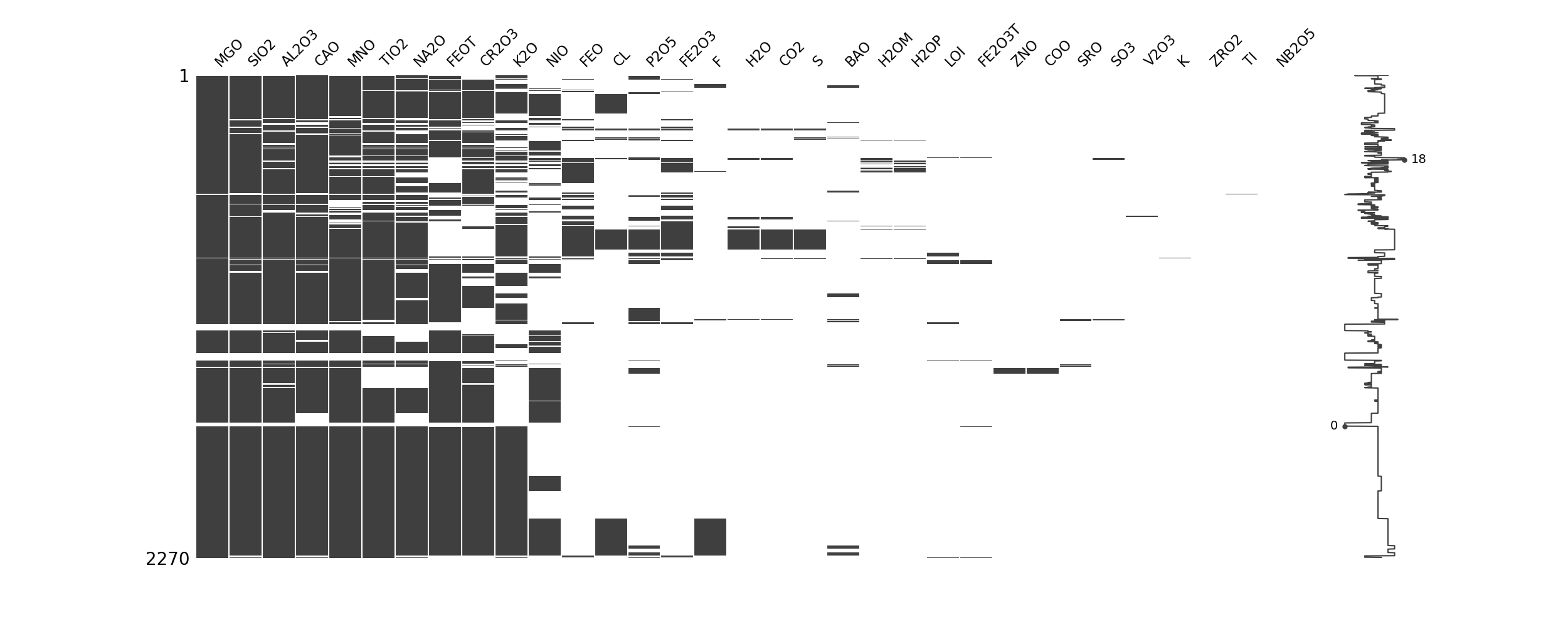
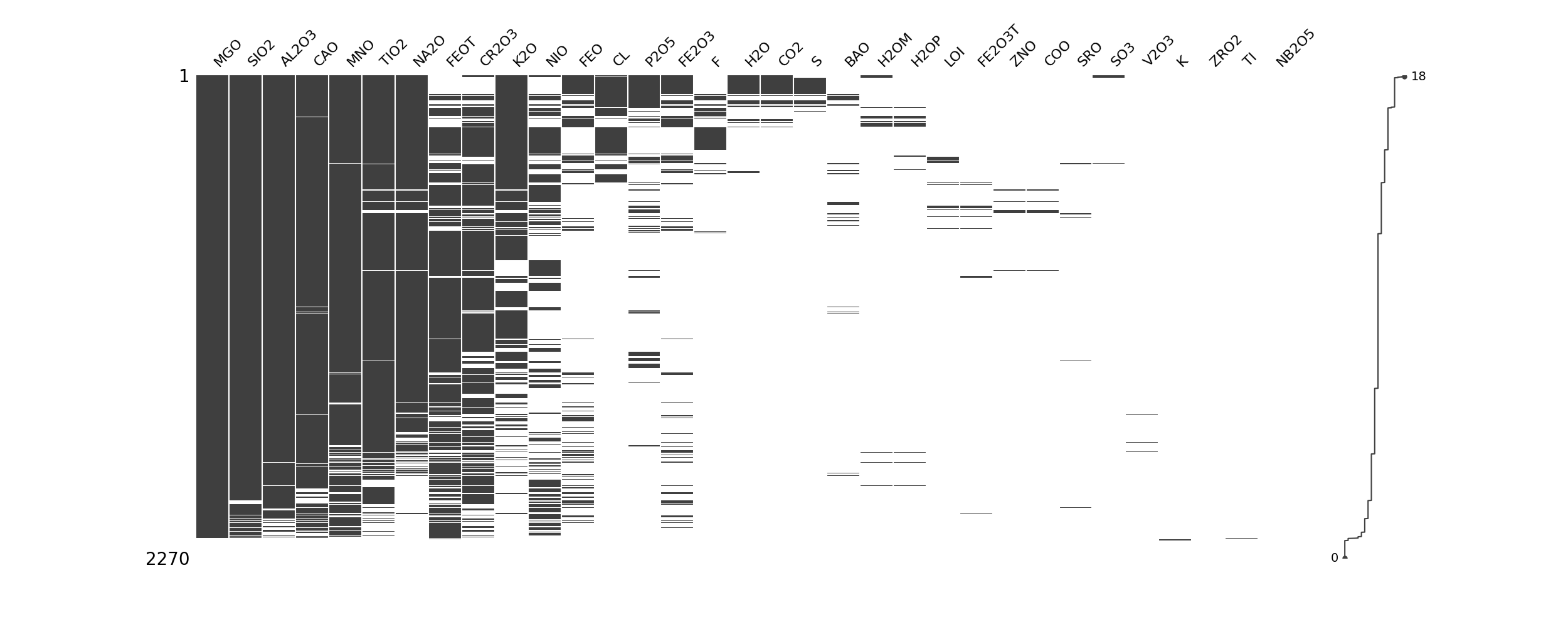
To get an overview of the completeness of the data, it can still be sorted by the zero values.
import missingno as msno
import pandas as pd
import matplotlib.pyplot as plt


data = pd.read_csv("path/to/Data.csv")

data_sorted_rows = data.loc[data.isnull().sum(axis=1).sort_values(ascending=True).index]
data_sorted_rows = data_sorted_rows.reset_index(drop=True)

null_counts = data_sorted_rows.isnull().sum()
sorted_columns = null_counts.sort_values(ascending=True).index
data_sorted_rows = data_sorted_rows[sorted_columns]

msno.matrix(data_sorted_rows)

plt.show()
Technique 2: Percentage list of missing data
Create a list with the percentages of missing values.
import numpy as np

# Iterate through each column in cols
for column in cols:
    # Calculate the percentage of missing values in the column
    missing_value_pct = np.mean(data[column].isnull())

    # Print column name and percentage of missing values
    print('Column: {}, Missing Values: {:.2f}%'.format(column, missing_value_pct * 100))
Output:

Column: SampleID, Missing Values: 0.00%
Column: AL2O3, Missing Values: 56.00%
Column: BA, Missing Values: 56.00%
Column: CAO, Missing Values: 59.00%
Column: CE, Missing Values: 56.00%
...
Column: Longitude, Missing Values: 0%
Column: Latitude, Missing Values: 0%
Column: Units, Missing Values: 26%
Column: Item_Group, Missing Values: 0%
Create a backup copy of the file/table
Before performing data cleansing, it is advisable to create a copy of the original and erroneous data to ensure the traceability of the cleansing and to guarantee an audit-proof procedure. Simply deleting the original data after the cleanup is not recommended, as this would make it impossible to verify possible sources of error. An alternative method, especially in the case of multiple cleanup runs, is to store the corrected value in an additional column or row. If there are a large number of columns and rows to be corrected, it may also make sense to create a separate table. The decision which method to choose depends on various factors, including the available storage space.
Data standardization
Some examples
Uniform Units of Measurement:
Ensure that all data are in the same units of measurement (e.g., ppm, ppb, mg/kg, etc.). This may require conversion of units to provide a consistent basis for comparison.
import pandas as pd

# Load your Dataset
data = pd.read_csv('path/to/Data.csv')

# Convert mg/kg to ppm (1 mg/kg = 1 ppm)
data['Element_in_mg/kg'] = data['Element_in_mg/kg'] * 1
data.rename(columns={'Element_in_mg/kg': 'Element_in_ppm'}, inplace=True)
Coordinate Systems:
Geochemical data are often tied to geographic locations, so it is important to use a uniform coordinate system (e.g., WGS84, UTM, etc.). This may require the conversion of coordinates between different systems.
import pandas as pd
import pyproj

# Load your Dataset
data = pd.read_csv('path/to/Data.csv')

# Define Coordinate system
in_proj = pyproj.Proj(proj='utm', zone=33, ellps='WGS84')
out_proj = pyproj.Proj(proj='latlong', datum='WGS84')

# Convert your coordinates
data['Longitude'], data['Latitude'] = pyproj.transform(in_proj, out_proj, data['X'].values, data['Y'].values)
Consistent Sample Identifiers:
Ensure that all samples are labeled with consistent names to avoid confusion and potential errors in data analysis. This may include replacing abbreviations or standardizing naming schemes.
import pandas as pd

# Load your Dataset
data = pd.read_csv('path/to/Data.csv')

# Replace abbreviations in the "Item_Group" column
data['Item_Group'] = data['Item_Group'].replace({'mj': 'Major', 'ree': 'Rare Earth Elements', 'te': 'Trace Elements'})
Unification of analytical methods:
Geochemical data can be obtained by a variety of analytical methods. To ensure comparability, it is helpful to standardize the data based on a common analytical method or at least to clearly document the methods used.
import pandas as pd

# Load your Dataset
data = pd.read_csv('path/to/Data.csv')

# Document the analysis method for each column
analysis_methods = {
    'AL2O3': 'XRF',
    'BA': 'ICP-MS',
    # ...
}

data['Analysis_Method'] = data.columns.map(analysis_methods)
Unification of detection limits:
Different analyses have different detection limits. To make the data more comparable, it may be useful to mark all values below a certain detection limit as “undetectable” or “below detection limit”.
import pandas as pd

# Load your Dataset
data = pd.read_csv('path/to/Data.csv')

# Set values below the detection limit to "not detectable"
detection_limit = 0.01
data[data < detection_limit] = 'not detectable'
Quality Control and Assurance:
Establishing standard procedures for quality control and assurance can help improve the accuracy and reliability of data. This includes reviewing sampling, analytical procedures, and data entry.
import pandas as pd

# Load your Dataset
data = pd.read_csv('path/to/Data.csv')

# Check if all necessary columns are present
required_columns = ['SampleID', 'AL2O3', 'BA', 'Longitude', 'Latitude']
missing_columns = set(required_columns) - set(data.columns)
if missing_columns:
    print(f'Missing columns: {missing_columns}')

# Check for duplicates in the "SampleID" column
duplicate_sample_ids = data[data.duplicated(subset='SampleID', keep=False)]
if not duplicate_sample_ids.empty:
    print(f'Duplicate in SampleID: {duplicate_sample_ids["SampleID"].tolist()}')
Data Types - Technical level
Data type 1: Inconsistent data
There may be additional strings concatenated to some numeric values that we need to remove. For this we define a function that removes these specific strings:
def remove_string(x):
	if type(x) is str:
		return x.replace('string', '')
	else:
		return x
Here ‘string’ can be removed in the replace function with the desired string.
Depending on the dataset it can be very helpful to get the datatypes of each column:
df = pd.read_csv("/path/to/csv")
df.dtypes
output:

SampleID int64
AL2O3 float64
BA float64
CAO float64
CE float64
CO float64
CR float64
CR2O3 float64
CS float64
DY float64
ER float64
EU float64
...
Certain values in the columns may be defined as objects, although we need numeric ones. For this we can redefine them:
df["LA"] = pd.to_numeric(df["LA"])
df["NA2O"] = pd.to_numeric(df["NA2O"])
df.dtypes
Output:

SampleID int64
AL2O3 float64
BA float64
CAO float64
CE float64
CO float64
CR float64
CR2O3 float64
CS float64
DY float64
ER float64
EU float64
The same applies to column names or categorical values, here you often have to pay attention to upper and lower case.
# make everything lower case.
df['author_lower'] = df['LA'].str.lower()
df['author_lower'].value_counts(dropna=False)
For example, all author names are all lowercase, in case it is necessary for the upcoming analysis method.
A common hurdle with processing the data is that some or all of the features are not recognized. This occurs when you have columns with strings. Here, it can happen that one or more spaces are placed before or after that of the string. These should be removed:
# getting all the columns with string/mixed type values
str_cols = list(df.columns)
str_cols.remove('MNO')

# removing leading and trailing characters from columns with str type
for i in str_cols:
	df[i] = df[i].str.strip()
In the context of the Tidy Data structure it becomes indispensable to pay attention to these hurdles.
Before you want to set out to remove missing values or possibly even use complex methods to fill them in, take a closer look at the data set. You may be able to extract missing values based on valid information from the dataset.
Data type 2: Irregular data (outliers)
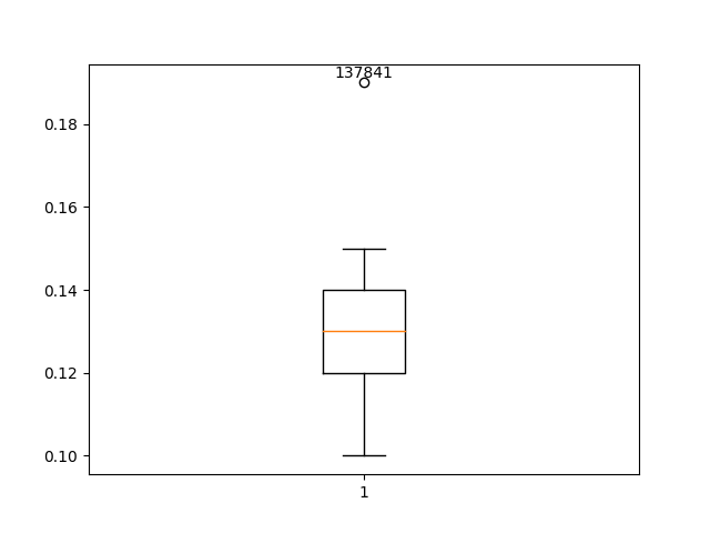
If the values are numeric, we can use a histogram and boxplot to detect outliers. The disadvantage of boxplots can be that numerical outliers can be very pronounced and that this is not correctly represented in the boxplot. However, the advantage of boxplots is that you can quickly visually see if the values are normally distributed.
Boxplot of observations
import pandas as pd
import matplotlib.pyplot as plt

# read in data
df = pd.read_csv("restructed_data.csv")

# draw boxplot and get quartiles
fig, ax = plt.subplots()
ax.boxplot(df['MNO'])

# identify outliers
q1 = df['MNO'].quantile(0.25)
q3 = df['MNO'].quantile(0.75)
iqr = q3 - q1

lower_bound = q1 - 1.5 * iqr
upper_bound = q3 + 1.5 * iqr

outliers_indices = [i for i, value in enumerate(df['MNO']) if value < lower_bound or value > upper_bound]
outliers_y = [value for value in df['MNO'] if value < lower_bound or value > upper_bound]

# find sampleIDs of outliers
outliers_sample_ids = df.iloc[outliers_indices]['SampleID'].tolist()

# add SampleIDs as text to the boxplot
for index, outlier, sample_id in zip(outliers_indices, outliers_y, outliers_sample_ids):
    ax.annotate(str(sample_id), (1, outlier), textcoords="offset points", xytext=(0, 3), ha='center')

# add x-axis labels
ax.set_xticks([1]) # Here we set the position of the x-tick
ax.set_xticklabels(['MnO']) # Here we set the label of the x-tick

plt.show()
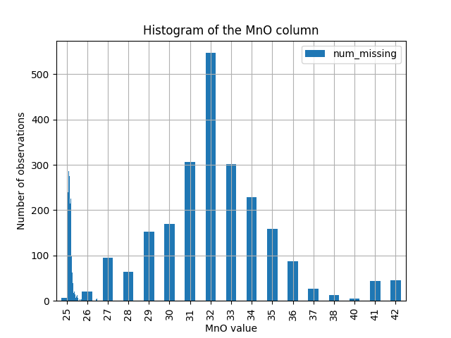
Histogram of observations
import pandas as pd
import matplotlib.pyplot as plt

# Load your Dataset
data = pd.read_csv('path/to/Data.csv')
column_name = 'MNO' # replace 'column_name' with the actual column name

# create histogram of the selected column
data[column_name].hist(bins=50)
plt.xlabel(column_name)
plt.ylabel('Number of observations')
plt.title(f'Histogram of {column_name} column')
plt.savefig('Hist_mno.png')
plt.show()
Descriptive statistics
Then we can use the methods of descriptive statistics. Here it can be helpful to find out whether a characteristic and its values are normally distributed or not. For example, the Shapiro-Wilk test can be used for this purpose.
import pandas as pd
import numpy as np
from scipy import stats

# Load your Dataset
data = pd.read_csv('path/to/Data.csv')

# exclude columns
exclude_columns = ['SampleID', 'Longitude', 'Latitude', 'Units', 'Item_Group']
selected_columns = [col for col in data.columns if col not in exclude_columns]

# perform Shapiro-Wilk test for each selected column
alpha = 0.05

for column_name in selected_columns:
    selected_data = data[column_name]

    # check if the data has a value range greater than zero
    if np.ptp(selected_data) > 0:
        statistic, p_value = stats.shapiro(selected_data)

        print(f"\nShapiro-Wilk test for column '{column_name}':")
        print(f" statistics: {statistic}")
        print(f" p-value: {p_value}")

        if p_value > alpha:
            print(f" The data in column '{column_name}' appears to be normally distributed (H0 not rejected).")
        else:
            print(f" The data in column '{column_name}' does not appear to be normally distributed (H0 rejected).")
    else:
        print(f"\nThe data in column '{column_name}' has a range of zero. Shapiro-Wilk test is not performed.")
Shapiro-Wilk test for column 'AL2O3':
  Statistic: 0.9374846816062927
  p-value: 0.4661906361579895
  Data in column 'AL2O3' appear to be normally distributed (H0 not rejected).

Shapiro-Wilk test for column 'BA':
  Statistic: 0.8701132535934448
  p-value: 0.0655660405755043
  Data in column 'BA' appear to be normally distributed (H0 not rejected).

Shapiro-Wilk test for column 'CAO':
  Statistic: 0.777439534664154
  p-value: 0.005249298643320799
  Data in column 'CAO' does not appear to be normally distributed (H0 rejected).
Further methods like IQR can be used to statistically distinguish between outliers and errors. Here, of course, the outliers must be assessed and decide how to deal with outliers depending on the data set and the goal of the project.Outliers are innocent until proven guilty. Other than that, they should not be removed unless there is a valid reason to do so.
Suitable methods are still to use to detect anomalies/outliers algorithms. Two are presented here that are included in sklearn by default:
LOF - Local Outlier Factors
import pandas as pd
from sklearn.neighbors import LocalOutlierFactor
from sklearn.preprocessing import StandardScaler

# Load your Dataset
data = pd.read_csv('path/to/Data.csv')

# remove the columns you don't want to analyze
data = data.drop(columns=["SampleID", "Longitude", "Latitude", "Units", "Item_Group"])

# scale the data to make sure that all columns have a similar impact
scaler = StandardScaler()
scaled_data = scaler.fit_transform(data)

# Create the Local Outlier Factor model
lof = LocalOutlierFactor(n_neighbors=12, contamination=0.05) # set the desired parameters

# Train the model and get the predictions
outlier_predictions = lof.fit_predict(scaled_data)

# Add the predictions to your original data set
data["outlier"] = outlier_predictions

# outliers are marked with -1, inliers with 1
outliers = data[data["outlier"] == -1]
inliers = data[data["outlier"] == 1]

print("Outliers:")
print(outliers)
print("Inliers:")
print(inliers)
Outliers:
   AL2O3   BA   CAO    CE     CO  ...     V    Y     YB    ZR  outlier
0   2.68  8.4  2.32  4.31  107.0  ...  61.0  0.0  0.291  2.15       -1

[1 rows x 45 columns]
Inliers:
    AL2O3     BA   CAO     CE     CO  ...     V       Y     YB     ZR  outlier
1    2.21  39.90  0.02  3.940  107.0  ...  34.0   0.470  0.047   0.73        1
2    1.02  30.40  0.83  3.850  107.0  ...  37.0   0.490  0.052   0.32        1
3    1.08  47.70  0.95  4.290  111.0  ...  35.0   0.297  0.036   0.43        1
4    2.59  17.60  0.04  1.610  114.0  ...  30.0   0.000  0.037   0.48        1
5    3.13   0.64  0.04  5.900   82.0  ...  77.0  10.800  1.100  24.70        1
6    3.65  40.00  3.73  1.410   95.0  ...  83.0   0.000  0.390   4.40        1
7    3.99  21.20  4.28  3.390   98.0  ...  77.0   4.780  0.530   8.70        1
8    4.49   1.39  0.04  0.390  104.0  ...  75.0   0.000  0.380   3.53        1
9    4.28   0.09  0.03  0.950  102.0  ...  82.0  17.100  1.960  13.00        1
10   3.42   0.83  3.24  0.261  103.0  ...  74.0   3.270  0.390   2.70        1
11   3.13   7.00  0.00  0.750    0.0  ...  68.0   0.000  0.330   2.65        1
Isolation Forest
import pandas as pd
from sklearn.ensemble import IsolationForest
from sklearn.preprocessing import StandardScaler

# Load your Dataset
data = pd.read_csv('path/to/Data.csv')

# remove the columns you don't want to analyze
data = data.drop(columns=["SampleID", "Longitude", "Latitude", "Units", "Item_Group"])

# scale the data to make sure that all columns have a similar impact
scaler = StandardScaler()
scaled_data = scaler.fit_transform(data)

# Create the isolation forest model
isolation_forest = IsolationForest(contamination=0.05) # set the desired proportion of expected outliers

# Train the model and get the predictions
outlier_predictions = isolation_forest.fit_predict(scaled_data)

# Add the predictions to your original dataset
data["outlier"] = outlier_predictions

# outliers are marked with -1, inliers with 1
outliers = data[data["outlier"] == -1]
inliers = data[data["outlier"] == 1]

print("Outliers:")
print(outliers)
print("Inliers:")
print(inliers)
Outliers:
   AL2O3    BA   CAO   CE    CO      CR  ...      U     V     Y   YB    ZR  outlier
5   3.13  0.64  0.04  5.9  82.0  5230.0  ...  0.127  77.0  10.8  1.1  24.7       -1

[1 rows x 45 columns]
Inliers:
    AL2O3     BA   CAO     CE     CO  ...     V       Y     YB     ZR  outlier
0    2.68   8.40  2.32  4.310  107.0  ...  61.0   0.000  0.291   2.15        1
1    2.21  39.90  0.02  3.940  107.0  ...  34.0   0.470  0.047   0.73        1
2    1.02  30.40  0.83  3.850  107.0  ...  37.0   0.490  0.052   0.32        1
3    1.08  47.70  0.95  4.290  111.0  ...  35.0   0.297  0.036   0.43        1
4    2.59  17.60  0.04  1.610  114.0  ...  30.0   0.000  0.037   0.48        1
6    3.65  40.00  3.73  1.410   95.0  ...  83.0   0.000  0.390   4.40        1
7    3.99  21.20  4.28  3.390   98.0  ...  77.0   4.780  0.530   8.70        1
8    4.49   1.39  0.04  0.390  104.0  ...  75.0   0.000  0.380   3.53        1
9    4.28   0.09  0.03  0.950  102.0  ...  82.0  17.100  1.960  13.00        1
10   3.42   0.83  3.24  0.261  103.0  ...  74.0   3.270  0.390   2.70        1
11   3.13   7.00  0.00  0.750    0.0  ...  68.0   0.000  0.330   2.65        1
Depending on the specific goals of a study and the available data, these and other algorithms and methods can help extract the information and insights needed to answer your scientific questions.
Data Types - Meaning level
Type 1: Non-informative/repetitive
To identify such data types, we can create a lists of features with a high percentage of the same value. A suitable example would be to show us columns where over 95% of the rows have the same value.
import pandas as pd

# Load the data
data = pd.read_csv('path/to/Data.csv')

# Calculate the number of rows in the dataset
total_rows = data.shape[0]

# Create a list to hold columns with low information density
low_info_columns = []

# Go through each column in the dataset
for column in data.columns:
    # Count the number of unique values in the column, including NaN values
    unique_counts = data[column].value_counts(dropna=False)

    # Calculate the percentage of the most common value
    dominant_value_pct = (unique_counts / total_rows).iloc[0]

    # If the percentage is more than 95%, add the column to the list and print relevant info
    if dominant_value_pct > 0.95:
        low_info_columns.append(column)
        print('Column: {0}, Dominant Value Percentage: {1:.5f}%'.format(column, dominant_value_pct * 100))
        print(unique_counts)
        print()

# Create a new DataFrame with the columns of low information density
low_info_data = data[low_info_columns]

# Save the new DataFrame as a CSV file
low_info_data.to_csv("low_information_data.csv", index=False)
K: 100.00000%
0.0 12
name: K, dtype: int64

RB87_SR86: 100.00000%
0.0 12
Name: RB87_SR86, dtype: int64

SR87_SR86: 100.00000%
0.0 12
Name: SR87_SR86, dtype: int64

Longitude: 100.00000%
38.21 12
Name: Longitude, dtype: int64

Latitude: 100.00000%
3.9 12
Name: Latitude, dtype: int64
In such cases the individual columns/values must be examined individually whether they are informative or not. It is important to find out the decisive reason why the values are repeated. If the values are not informative, they can be removed.
Type 2: Irrelevant data type
The quality of the data collected plays an essential role in providing meaningful information for the successful implementation of a project. Characteristics that are not related to the project’s problem are irrelevant to the analysis.
A systematic examination of all available characteristics is required to determine their relevance. Characteristics that are not meaningful to the project goals should be removed from the analysis to ensure focused and purposeful results.
import pandas as pd

# Load your Dataset
df = pd.read_csv('path/to/Data.csv')

# remove row based on index n OR:
df = df.drop(n)

# remove column 'name' OR:
df = df.drop('MNO', axis=1)

# remove columns 'MNO' and 'FEO
df = df.drop(['MNO', 'FEO'], axis=1)
Type 3: Duplicates
Duplicate data exists when copies of the same observation are present. It often happens that there are several types of data in one column, which we have to handle separately. In this case we can use the split function:
splitted_columns = df['author, column'].str.split(',',expand=True)
splitted_columns
Followed by clearly mapping the new columns and removing the old column that contained multiple pieces of information:
df['author'] = splitted_columns[0]
df['column'] = splitted_columns[1]
df.head()
df.drop('author, column', axis=1, inplace=True)
df.head(15)
Duplicate Type 1
In geochemistry, datasets may contain duplicates where all variable values within an observation are the same. Identifying and removing such duplicates is an important step in data preparation to ensure the integrity and validity of statistical analyses.
# Considering 'MNO' column is unique, let's see the effect of removing it
deduplicated_data = df.drop(columns='MNO').drop_duplicates()

# Compare the shape before and after deduplication
print(f"Original DataFrame shape: {df.shape}")
print(f"Deduplicated DataFrame shape: {deduplicated_data.shape}")
Output:

Original DataFrame shape: (12, 49)
Deduplicated DataFrame shape: (12, 48)
Duplicate Type 2
In some cases, it is appropriate to weed out redundant records based on a set of specific, unique identifiers.
For example, in a geochemical context, it is extremely unlikely that two samples will be collected at exactly the same time and location, and will also have identical chemical compositions.
A grouping of essential characteristics can serve as unique identifiers for such samples. These include, for example, the time of sampling, geographic coordinates, pH, heavy metal and mineral content, and organic compound content. These characteristics can be used to identify and remove possible duplicates.
import pandas as pd

# Load your Dataset
df = pd.read_csv('path/to/Data.csv')

key = ['SampleID', 'AL2O3', 'FEO', 'FEOT', 'K', 'Longitude', 'Latitude']

df.fillna(-999).groupby(key)['SampleID'].count().sort_values(ascending=False).head(20)

df_dedupped2 = df.drop_duplicates(subset=key)

print(df)
print(df.shape)
print(df_dedupped2.shape)
    SampleID  AL2O3     BA   CAO  ...  Longitude  Latitude  Units  Item_Group
0     137833   2.68   8.40  2.32  ...      38.21       3.9    WT%          mj
1     137834   2.21  39.90  0.02  ...      38.21       3.9    WT%          mj
2     137835   1.02  30.40  0.83  ...      38.21       3.9    PPM         ree
3     137836   1.08  47.70  0.95  ...      38.21       3.9    PPM          te
4     137837   2.59  17.60  0.04  ...      38.21       3.9    WT%          mj
5     137838   3.13   0.64  0.04  ...      38.21       3.9    WT%          mj
6     137839   3.65  40.00  3.73  ...      38.21       3.9    PPM          te
7     137840   3.99  21.20  4.28  ...      38.21       3.9    PPM          te
8     137841   4.49   1.39  0.04  ...      38.21       3.9    WT%          mj
9     137842   4.28   0.09  0.03  ...      38.21       3.9    WT%          mj
10    137843   3.42   0.83  3.24  ...      38.21       3.9    WT%          mj
11    137844   3.13   7.00  0.00  ...      38.21       3.9    PPM         ree

[12 rows x 49 columns]

(12, 49)
(12, 49)
Scaling, transformation and normalization
Scaling and transformation refer to the fitting of data to a specific scale, such as in the range of 0-100 or 0-1. This can facilitate the presentation and interpretation of data, especially in reducing skewness and handling outliers. Examples of transformations include logarithm, square root, and inverse. Using these techniques can help optimize data visualization and improve comparability of data points within a dataset.
import pandas as pd
import numpy as np

# Load your Dataset
data = pd.read_csv('path/to/Data.csv')

# select numerical columns only
numerical_columns = data.select_dtypes(include=['number']).columns

# min-max scaling
data_min_max = data.copy()
data_min_max[numerical_columns] = (data[numerical_columns] - data[numerical_columns].min()) / (data[numerical_columns].max() - data[numerical_columns].min())

# standardization (Z-score normalization)
data_standardized = data.copy()
data_standardized[numerical_columns] = (data[numerical_columns] - data[numerical_columns].mean()) / data[numerical_columns].std()

# Logarithmic transformation
data_log = data.copy()
data_log[numerical_columns] = data[numerical_columns].apply(lambda x: x+1).apply(np.log) # x+1 to avoid errors with logarithm of 0

# square root transformation
data_sqrt = data.copy()
data_sqrt[numerical_columns] = data[numerical_columns].apply(np.sqrt)

# Inverse transformation
data_inverse = data.copy()
data_inverse[numerical_columns] = 1 / (data[numerical_columns] + 1e-9) # 1e-9 to avoid division by zero

# output transformed data sets
print("Min-Max scaled data:\n", data_min_max)
print("Standardized data:\n", data_standardized)
print("Logarithmically transformed data:\n", data_log)
print("Square root transformed data:\n", data_sqrt)
print("Inverse-transformed data:\n", data_inverse)
Min-Max scaled data:
     SampleID AL2O3 BA ...  Latitude Units Item_Group
0 0.000000 0.478386 0.174543 ...       NaN WT% mj
1 0.090909 0.342939 0.836169 ...       NaN WT% mj
2 0.181818 0.000000 0.636631 ...       NaN PPM ree
...

Standardized data:
     SampleID AL2O3 BA ...  Latitude Units Item_Group
0 -1.525426 -0.259611 -0.540761 ...       NaN WT% mj
1 -1.248075 -0.676764 1.246800 ...       NaN WT% mj
2 -0.970725 -1.732959 0.707694 ...       NaN PPM ree
...

Logarithmically transformed data:
      SampleID AL2O3 BA ...  Latitude Units Item_Group
0 11.833805 1.302913 2.240710 ...  1.589235 WT% mj
1 11.833813 1.166271 3.711130 ...  1.589235 WT% mj
2 11.833820 0.703098 3.446808 ...  1.589235 PPM ree
...

Square root transformed data:
       SampleID AL2O3 BA ...  Latitude Units Item_Group
0 371.258670 1.637071 2.898275 ...  1.974842 WT% mj
1 371.260017 1.486607 6.316645 ...  1.974842 WT% mj
2 371.261363 1.009950 5.513620 ...  1.974842 PPM ree
...

Inverse-transformed data:
     SampleID AL2O3 BA ...  Latitude Units Item_Group
0 0.000007 0.373134 0.119048 ...   0.25641 WT% mj
1 0.000007 0.452489 0.025063 ...   0.25641 WT% mj
2 0.000007 0.980392 0.032895 ...   0.25641 PPM ree
Cleaning the data
Missing values
Missing values in geochemical data can be handled in several ways:
- elimination, in which rows or columns with missing values are removed.
- imputation, where missing values are calculated based on existing data, using various methods such as statistical values, linear regression, or hot deck imputation.
- labeling, in which missing data are replaced with special values or categories to maintain the information content. It is important to distinguish between missing values, default values, and unknown values, and to consider the loss of information when deciding on a method.
Elimination:
import pandas as pd

# Load your Dataset
data = pd.read_csv('path/to/Data.csv')

# remove rows with missing values
data_cleaned_rows = data.dropna()

# remove columns with missing values
data_cleaned_columns = data.dropna(axis=1)
Imputation:
import pandas as pd
import numpy as np

# Load your Dataset
data = pd.read_csv('path/to/Data.csv')

# replace missing values with the median of the column
data_median_imputed = data.fillna(data.median())

# Example: Replace missing values in column 'AL2O3' with random values in the range of 2 standard deviations from the average
mean_AL2O3 = data['AL2O3'].mean()
std_AL2O3 = data['AL2O3'].std()
count_nan_AL2O3 = data['AL2O3'].isnull().sum()

rand_AL2O3 = np.random.randint(mean_AL2O3 - 2 * std_AL2O3, mean_AL2O3 + 2 * std_AL2O3, size=count_nan_AL2O3)
data['AL2O3'][data['AL2O3'].isnull()] = rand_AL2O3
Labeling:
import pandas as pd

# Load your Dataset
data = pd.read_csv('path/to/Data.csv')

# replace missing numeric values with 0
data_zero_filled = data.fillna(0)

# replace missing categorical values in 'Units' column with 'Missing
data_category_flagged = data.fillna({'Units': 'Missing'})
Verification
Verification should be performed both before and after scaling, transformation, and normalization. Performing verification before scaling ensures that the changes made in the data cleaning process are correct and will not have an unintended effect on the data. Performing verification after scaling, transformation, and normalization allows you to verify the quality and consistency of the scaled and transformed data and ensure that the methods used have not changed the data in an undesirable way.
Visualizations:
Re-create visualizations such as histograms, boxplots, or scatterplots to verify that the distribution of the data and the relationships between columns are as expected.
Check the number of missing values:
You can do this again with the heatmap or the list of percentages of missing values.
Sample check:
Manually check a few data points to make sure the values are correct and consistent.
Check data types:
df = pd.read_csv("/path/to/csv")
df.dtypes
Check the uniqueness of IDs or keys:
If your dataset contains an ID column or unique key, make sure there are no duplicates.
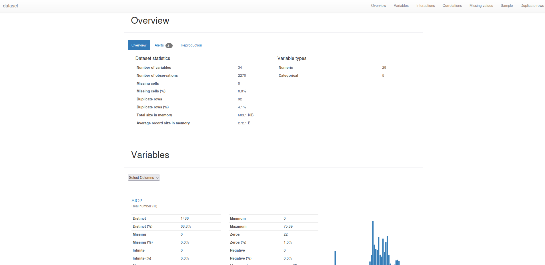
Statistical Summaries:
import pandas as pd
from ydata_profiling import ProfileReport

data = pd.read_csv("restructed_data.csv")

columns_to_ignore = ['SampleID', 'Units', 'Item_Group', 'Latitude', 'Longitude']
columns_to_profile = [col for col in data.columns if col not in columns_to_ignore]

profile = ProfileReport(data[columns_to_profile], title="dataset")
profile.to_file("dataset.html")
Documentation
Documentation of the data cleaning process is an essential part of processing geochemical data sets. Careful documentation helps to ensure transparency, traceability, and reproducibility of results. This is critical to maintaining scientific integrity and enhancing the credibility of research results. When documenting data cleaning related to geochemical datasets, there are several aspects to consider:
-
Describe the raw data: Document the source and extent of geochemical data, including analytical methods used, sampling processes, and initial dataset structure.
-
Determine Data Quality Requirements: Determine the data quality and consistency criteria required for your specific geochemical question and document these requirements.
-
Steps of the Data Cleaning Process: List a detailed description of all steps performed in the data cleaning process, such as identifying and removing outliers, correcting inconsistent data, standardizing units of measure, or removing duplicates.
-
Tools and Scripts Used: Document all Python libraries, functions, and scripts used in the Data Cleaning process to ensure reproducibility of results.
-
Decisions and Justifications: Explain the decisions made during the Data Cleaning process and provide the rationale for those decisions. This may include, for example, selecting specific thresholds for removing outliers or applying specific normalization procedures.
-
Changes and Impacts: Describe how the data cleaning steps performed affected the structure, volume, and quality of the geochemical data and, if applicable, show the impact of these changes on the results of your analysis.
-
Versioning and Change History: Maintain a change history of the various versions of your Data Cleaning scripts and documentation to facilitate collaboration and tracking of changes over time.
References
Walker, M. (2020) Python Data Cleaning Cookbook: Modern Techniques and Python Tools to Detect and Remove Dirty Data and Extract Key Insights. Packt Publishing.
pandas McKinney, W. (2010). “Data Structures for Statistical Computing in Python.” Proceedings of the 9th Python in Science Conference. pp. 56-61.
missingno Bilogur, (2018). Missingno: a missing data visualization suite. Journal of Open Source Software, 3(22), 547, https://doi.org/10.21105/joss.00547
matplotlib Hunter, J. D. (2007). “Matplotlib: A 2D Graphics Environment.” Computing in Science & Engineering, 9(3), pp. 90-95.
pyproj The pyproj library is a Python interface to PROJ (software for converting between geographic coordinate systems). The main reference would therefore be the PROJ software: PROJ contributors (2020). “PROJ, a library for cartographic projections and coordinate transformations.”
scipy Virtanen, P., Gommers, R., Oliphant, T. E., Haberland, M., Reddy, T., Cournapeau, D., … & SciPy 1.0 Contributors. (2020). “SciPy 1.0: fundamental algorithms for scientific computing in Python.” Nature methods, 17(3), pp. 261-272.
sklearn.ensemble.IsolationForest Liu, F. T., Ting, K. M., & Zhou, Z. H. (2008). “Isolation Forest.” 2008 Eighth IEEE International Conference on Data Mining. pp. 413-422.
sklearn.preprocessing.StandardScaler Pedregosa, F., Varoquaux, G., Gramfort, A., Michel, V., Thirion, B., Grisel, O., … & Vanderplas, J. (2011). “Scikit-learn: Machine Learning in Python.” Journal of Machine Learning Research, 12, pp. 2825–2830.
numpy Harris, C. R., Millman, K. J., van der Walt, S. J., Gommers, R., Virtanen, P., Cournapeau, D., … & SciPy 1.0 Contributors. (2020). “Array programming with NumPy.” Nature, 585(7825), pp. 357-362.
ydata_profiling.ProfileReport As of my knowledge cutoff in September 2021, there was no specific scientific literature available for the ydata_profiling library. It’s recommended to cite the library’s GitHub repository: https://github.com/ydataai/ydata-quality
License
CC BY-NC-SA 4.0 Licence
With this licence, you may use, modify and share the work as long as you credit the original author. However, you may not use it for commercial purposes, i.e. you may not make money from it. And if you make changes and share the new work, it must be shared under the same conditions.